Exponential Histograms: Better Data, Zero Configuration
Blog posts are not updated after publication. This post is more than a year old, so its content may be outdated, and some links may be invalid. Cross-verify any information before relying on it.
Histograms are a powerful tool in the observability tool belt. OpenTelemetry supports histograms because of their ability to efficiently capture and transmit distributions of measurements, enabling statistical calculations like percentiles.
In practice, histograms come in several flavors, each with its own strategy for representing buckets and bucket counts. The first stable metric release for OpenTelemetry included explicit bucket histograms, and now OpenTelemetry is introducing a new exponential bucket histogram option. This exciting new format automatically adjusts buckets to reflect measurements and is more compressed to send over the wire. This blog post dives into the details of exponential histograms, explaining how they work, the problem they solve, and how to start using them now.
Intro to metrics in OpenTelemetry
Before talking about exponential bucket histograms, let’s do a quick refresher on some general OpenTelemetry metrics concepts. If you’re already up to speed, skip ahead to Anatomy of a histogram.
Metrics represent aggregations of many measurements. We use them because it’s often prohibitively expensive to export and analyze measurements individually. Imagine the cost of exporting the time of each request for an HTTP server responding to one million requests per second! Metrics aggregate measurements to reduce data volume and retain a meaningful signal.
Like tracing (and someday soon logs), OpenTelemetry metrics are broken into the API and SDK. The API is used to instrument code. Application owners can use the API to write custom instrumentation specific to their domain, but more commonly they install prebuilt instrumentation for their library or framework. The SDK is used to configure what happens with the data collected by the API. This typically includes processing it and exporting it out of process for analysis, often to an observability platform.
The API entry point for metrics is the meter provider. It provides meters for different scopes, where a scope is just a logical unit of application code. For example, instrumentation for an HTTP client library would have a different scope and therefore a different meter than instrumentation for a database client library. You use meters to obtain instruments. You use instruments to report measurements, which consist of a value and set of attributes. This Java code snippet demonstrates the workflow:
OpenTelemetry openTelemetry = // declare OpenTelemetry instance
Meter meter = openTelemetry.getMeter("my-meter-scope");
DoubleHistogram histogram =
    meter
        .histogramBuilder("my-histogram")
        .setDescription("The description")
        .setUnit("ms")
        .build();
histogram.record(10.2, Attributes.builder().put("key", "value").build());
The SDK provides implementations of meter provider, meter, and instruments. It aggregates measurements reported by instruments and exports them as metrics according to the application configuration.
There are currently six types of instruments in OpenTelemetry metrics: counter, up down counter, histogram, async counter, async up down counter, and async gauge. Carefully consider which instrument type to select, since each implies certain information about the nature of the measurements it records and how they are analyzed. For example, use a counter when you want to count things and when the sum of the things is more important than their individual values (such as tracking the number of bytes sent over a network). Use a histogram when the distribution of measurements is relevant for analysis. For example, a histogram is a natural choice for tracking response times for HTTP servers, because it’s useful to analyze the distribution of response times to evaluate SLAs and identify trends. To learn more, see the guidelines for instrument selection.
I mentioned earlier that the SDK aggregates measurements from instruments. Each instrument type has a default aggregation strategy (or simply aggregation) that reflects the intended use of the measurements as implied by the instrument type selection. For example, counters and up down counters aggregate to a sum of their values. Histograms aggregate to a histogram aggregation. (Note that histogram is both a type of instrument and an aggregation.)
Anatomy of a histogram
What is a histogram? Putting OpenTelemetry aside for a moment, we’re all somewhat familiar with histograms. They consist of buckets and counts of occurrences within those buckets.
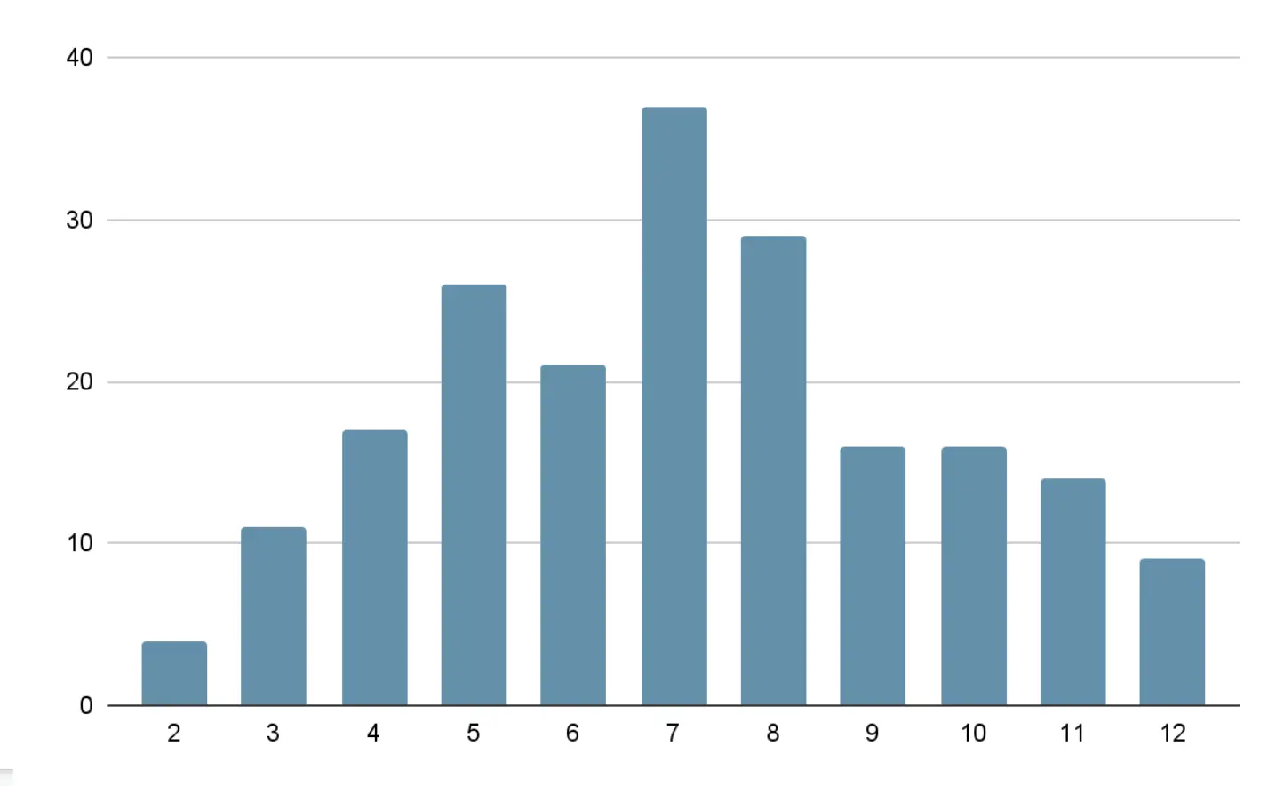
For example, a histogram could track the number of times a particular number was rolled with the sum of two six-sided dice, with one bucket for each possible outcome, from 2-12. Over a large number of rolls, you expect the 7 bucket to have the highest count because you are more likely to roll a combined total of 7, and the 2 and 12 buckets to have the least because these are the least likely rolls, as shown in this example histogram.
OpenTelemetry has two types of histograms. Let’s start with the relatively simpler explicit bucket histogram. It has buckets with boundaries explicitly defined during initialization. For example, if you configure it with boundaries [0,5,10], there are N+1 buckets with boundaries (-∞, 0],(0,5],(5,10], (10,+∞]. Each bucket tracks the number of occurrences of values within its boundaries. Additionally, the histogram tracks the sum of all values, the count of all values, the maximum value, and the minimum value. See the opentelemetry-proto for the complete definition.
Before we talk about the second type of histogram, pause and think about some of the questions you can answer when data is structured like this. Assuming you’re using a histogram to track the number of milliseconds it took to respond to a request, you can determine:
- The number of requests.
- The minimum, maximum, and average request latency.
- The percentage of requests that had latency less than a particular bucket boundary. For example, if buckets boundaries are [0,5,10], you can take the sum of the counts of buckets (-∞,0],(0,5],(5,10], and divide by the total count to determine the percentage of requests that took less than 10 milliseconds. If you have an SLA that 99% of requests must be resolved in more than 10 milliseconds, you can determine whether or not you met it.
- Patterns, by analyzing the distribution. For example, you might find that most requests resolve quickly but a small number of requests take a long time and bring down the average.
The second type of OpenTelemetry histogram is the exponential bucket histogram. Exponential bucket histograms have buckets and bucket counts, but instead of explicitly defining the bucket boundaries, the boundaries are computed based on an exponential scale. More specifically, each bucket is defined by an index i and has bucket boundaries (base**i, base**(i+1)], where base**i means that base is raised to the power of i. The base is derived from a scale factor that is adjustable to reflect the range of reported measurements and is equal to 2**2**-scale. Bucket indexes must be continuous, but a non-zero positive or negative offset can be defined. For example, at scale 0, base = 2**2**-0 = 2 , and the bucket boundaries for indexes [-2,2] are defined as (.25,.5],(.5,1],(1,2],(2,4],(4,8]. By adjusting the scale, you can represent both large and small values. Like explicit bucket histograms, exponential bucket histograms also track the sum of all values, the count of all values, the maximum value, and the minimum value. See the opentelemetry-proto for the complete definition.
Why use exponential bucket histograms
On the surface, exponential bucket histograms don’t seem very different from explicit bucket histograms. In reality, their subtle differences yield dramatically different results.
Exponential bucket histograms are a more compressed representation. Explicit bucket histograms encode data with a list of bucket counts and a list of N-1 bucket boundaries, where N is the number of buckets. Each bucket count and bucket boundary is an 8-byte value, so an N bucket explicit bucket histogram is encoded as 2N-1 8-byte values.
In contrast, bucket boundaries for exponential bucket histograms are computed based on a scale factor and an offset defining the starting index of the buckets. Each bucket count is an 8-byte value, so an N bucket exponential bucket histogram is encoded as N+2 8-byte values (N bucket counts and 2 constants). Of course, both of these representations are commonly compressed when sent over a network, so further size reduction is likely, but exponential bucket histograms contain fundamentally less information.
Exponential bucket histograms are basically configuration-free. Explicit bucket histograms need an explicitly defined set of bucket boundaries that need to be configured somewhere. A default set of boundaries is provided, but use cases of histograms vary wildly enough that it’s likely you’ll need to adjust the boundaries to better reflect your data. The view API helps, with mechanisms to select specific instruments and redefine the explicit bucket histogram aggregation bucket boundaries.
In contrast, the only configurable parameter of exponential bucket histograms is the number of buckets, which defaults to 160 for positive values. The implementation automatically chooses the scale factor, based on the range of values recorded and the number of buckets available to maximize the bucket density around the recorded values. I can’t overstate how useful this is.
Exponential bucket histograms capture a high-density distribution of values automatically adjusted for the scale and range of measurements, with no configuration. The same histogram that captures nanosecond scale measurements is equally good at capturing second scale measurements. They retain fidelity regardless of scale.
Consider the scenario of capturing HTTP request time milliseconds. With an explicit bucket histogram, you make guesses on bucket boundaries which you hope will accurately capture the distribution of values. But if conditions change and latency spikes, your assumptions might not hold and all values could be lumped together. Suddenly, you’ve lost visibility into the distribution of data. You know latency is high overall. But you can’t know how many requests are high but tolerable versus terribly slow. In contrast, with an exponential bucket histogram, the scale automatically adjusts to the latency spikes to choose the optimal range of buckets. You retain insight into the distribution, even with a large range of measurement values.
Example scenario: explicit bucket histograms vs. exponential bucket histograms
Let’s bring everything together with a proper demonstration comparing explicit bucket histograms to exponential bucket histograms. I’ve put together some example code that simulates tracking response time to an HTTP server in milliseconds. It records one million samples to an explicit bucket histogram with the default buckets, and to an exponential bucket histogram with a number of buckets that produces roughly the same size of OTLP -encoded, Gzip-compressed payload as the explicit bucket defaults. Through trial and error, I determined that ~40 exponential buckets produce an equivalent payload size to the default explicit bucket histogram with 11 buckets. (Your results may vary.)
I wanted the distribution of samples to reflect what we might see in an actual HTTP server, with bands of response times corresponding to different operations. It will look something like this example:
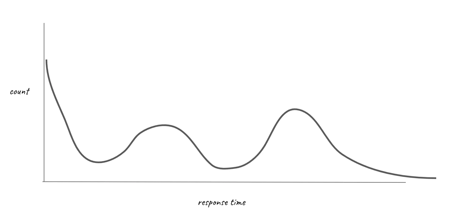
To achieve this, I used a variety of different probability distributions, each corresponding to different bands in the curve, and each accounting for some percentage of the samples.
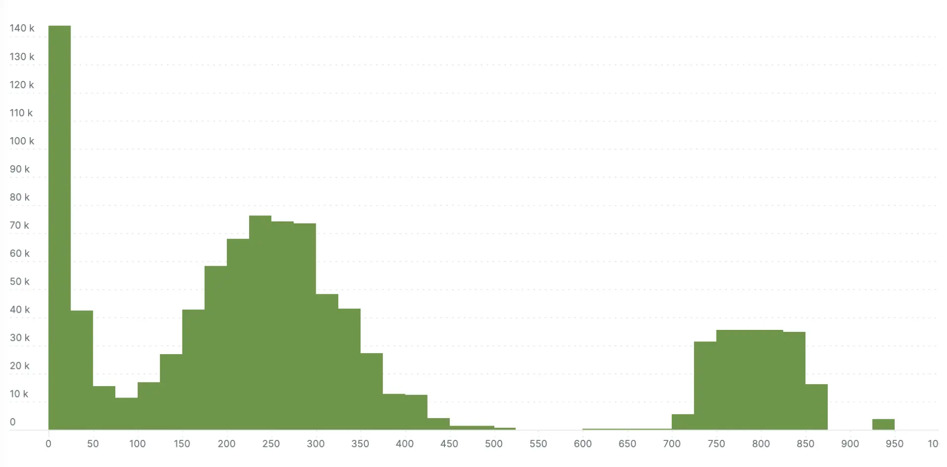
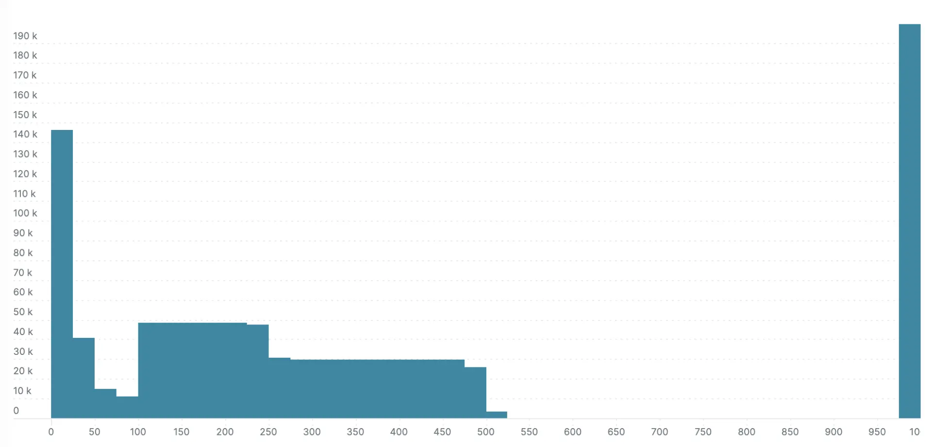
I ran the simulation, and exported the histograms via to compare the explicit bucket histogram to the exponential bucket histogram. The next two charts show the results. The exponential bucket histogram has significantly more detail, which simply isn’t available with the more limited buckets of the explicit bucket histogram.
Note: These visualizations are from the New Relic platform, which I used because they employ me, and it’s the easiest way for me to visualize histograms. Every platform will have its own mechanism for storing and retrieving histograms, which typically perform some lossy translation of buckets into a normalized storage format—New Relic is no exception. Additionally, the visualization doesn’t clearly delineate buckets, which causes adjacent buckets with the same count to appear as a single bucket.
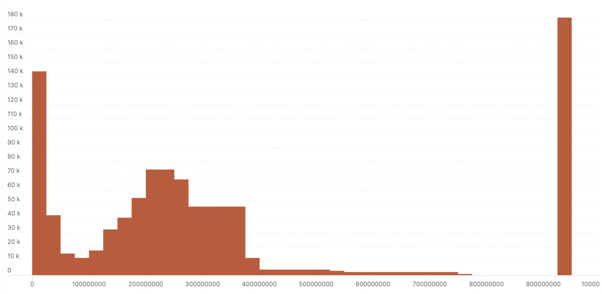
Here’s the millisecond scale exponential bucket histogram:
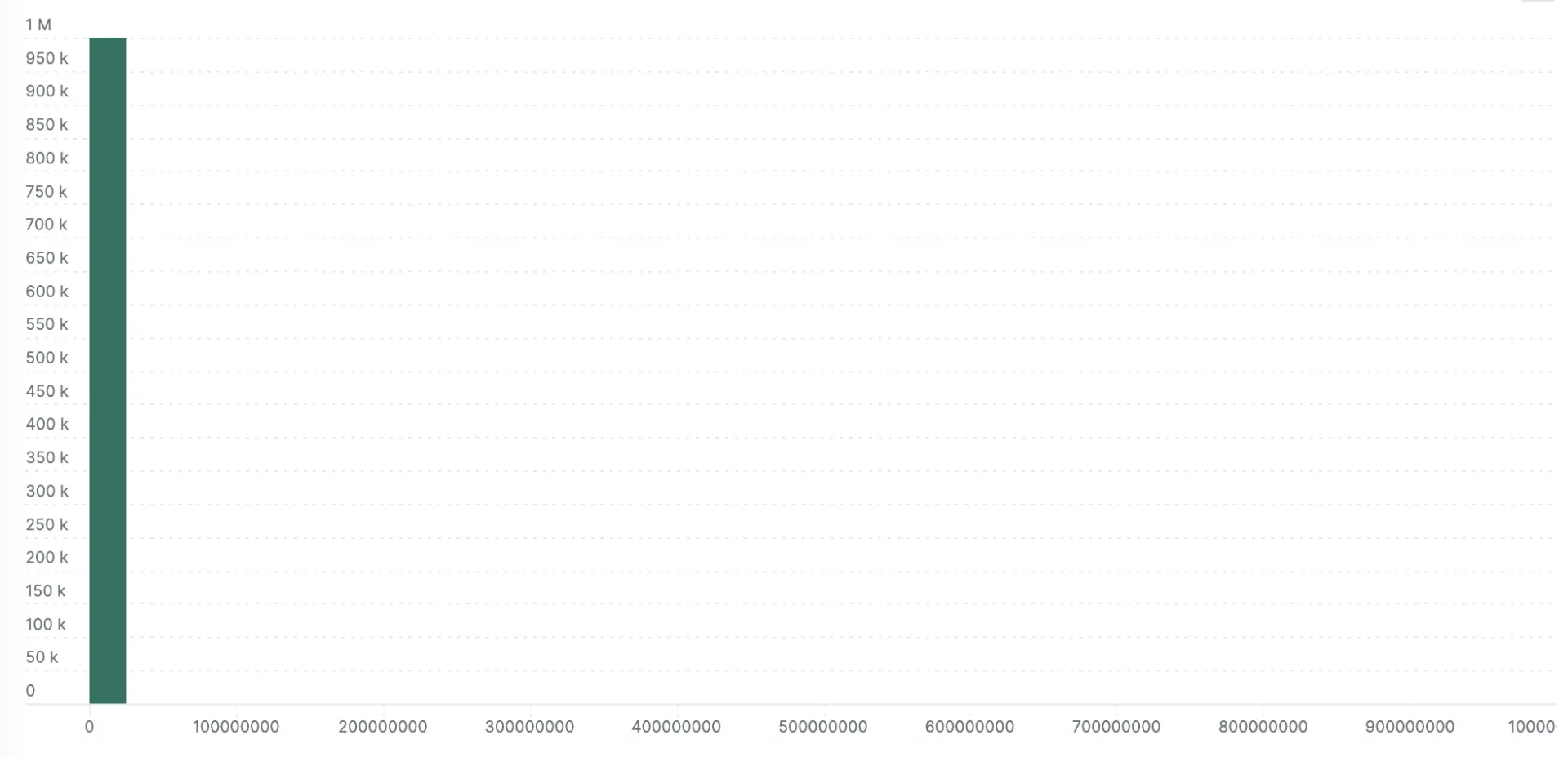
Here’s the millisecond scale explicit bucket histogram:
This demonstration is fairly generous to the explicit bucket histogram because I choose to report values in an optimum range for the default buckets (for example, 0 to 1000). The next two examples show what happens when the same values are recorded in nanosecond precision instead of milliseconds (all values are multiplied by 106). This is where the no-configuration autoscaling nature of exponential bucket histograms really shines. Left with the default explicit bucket boundaries, all the samples fall into a single bucket with the explicit bucket histogram. The exponential variety loses some definition compared to the millisecond version in the previous example, but you can still see the response time bands.
Here’s the nanosecond scale exponential bucket histogram:
Here’s the nanosecond scale explicit bucket histogram:
Next steps
Exponential bucket histograms are a powerful new tool for metrics. While implementations are still in progress at the time of publishing this post, you’ll definitely want to enable them when you’re using OpenTelemetry metrics.
If you’re using opentelemetry-java (and eventually other languages), the easiest way to enable exponential bucket histograms is by setting the environment variable with this command:
export OTEL_EXPORTER_OTLP_METRICS_DEFAULT_HISTOGRAM_AGGREGATION=exponential_bucket_histogram
For instructions on enabling in other languages, check the relevant documentation on instrumentation or github.com/open-telemetry.
A version of this article was originally posted on the New Relic blog.